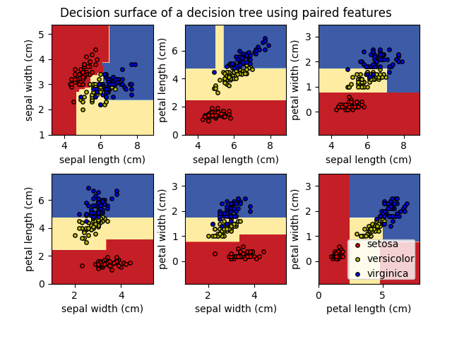
Plot the decision surface of a decision forest on the iris dataset

Plot the decision surface of a decision forest trained on pairs of features of the iris dataset based on scikit-learn’s Plot the decision surface of a decision tree on the iris dataset.

# Modified using koho's DecisionForestClassifier by AI Werkstatt

import numpy as np
import matplotlib.pyplot as plt

from sklearn.datasets import load_iris

from koho.sklearn import DecisionForestClassifier

# Parameters
n_classes = 3
plot_colors = "ryb"
plot_step = 0.02

# Load data
iris = load_iris()

for pairidx, pair in enumerate([[0, 1], [0, 2], [0, 3],
                                [1, 2], [1, 3], [2, 3]]):
    # We only take the two corresponding features
    X = iris.data[:, pair]
    y = iris.target

    # Train
    clf = DecisionForestClassifier(random_state=0).fit(X, y)

    # Plot the decision boundary
    plt.subplot(2, 3, pairidx + 1)

    x_min, x_max = X[:, 0].min() - 1, X[:, 0].max() + 1
    y_min, y_max = X[:, 1].min() - 1, X[:, 1].max() + 1
    xx, yy = np.meshgrid(np.arange(x_min, x_max, plot_step),
                         np.arange(y_min, y_max, plot_step))
    plt.tight_layout(h_pad=0.5, w_pad=0.5, pad=2.5)

    Z = clf.predict(np.c_[xx.ravel(), yy.ravel()])
    Z = Z.reshape(xx.shape)
    cs = plt.contourf(xx, yy, Z, cmap=plt.cm.RdYlBu)

    plt.xlabel(iris.feature_names[pair[0]])
    plt.ylabel(iris.feature_names[pair[1]])

    # Plot the training points
    for i, color in zip(range(n_classes), plot_colors):
        idx = np.where(y == i)
        plt.scatter(X[idx, 0], X[idx, 1], c=color, label=iris.target_names[i],
                    cmap=plt.cm.RdYlBu, edgecolor='black', s=15)

plt.suptitle("Decision surface of a decision tree using paired features")
plt.legend(loc='lower right', borderpad=0, handletextpad=0)
plt.axis("tight")
plt.show()